Getting started with psychHypergraph

What this tutorial covers

psychHypergraph constructs hypergraphs whose hyperedges represent selected groups of variables with redundancy-dominated or synergy-dominated statistical dependence. Unlike an ordinary edge, a hyperedge can contain more than two variables. The package uses O-information to describe the balance between redundancy and synergy (Rosas et al., 2019), then applies statistical screening before retaining candidate variable groups as hyperedges, drawing on the workflows of Marinazzo et al. (2024) and Possenti et al. (2026).

This tutorial follows a complete analysis of personality items: prepare the data, construct a hypergraph, inspect the results, visualize the hyperedges, calculate node degree, and explore node clusters. The companion vignette, Customize your own workflow, shows how to work with the individual modules and supply your own candidates.

The full example involves many resampling operations. The construction code is shown but is not evaluated when this vignette is built. Instead, the figures and tables use a saved reference fit distributed with the package. You can run the construction code yourself to repeat the analysis. The reference run used only 100 permutations and 100 bootstrap samples for demonstration. For a research analysis, increase these numbers, for example to at least 1,000 as an initial setting, and examine Monte Carlo precision and interval stability.

1. Load the packages and data

library(psychHypergraph)
library(psych)

data(bfi)
data_bfi <- bfi[, 1:25]

dim(data_bfi)
#> [1] 2800   25

The bfi dataset contains responses from 2,800 participants. We select the first 25 columns, which are personality items, and leave out the demographic variables. Rows are participants and columns are items. Each item uses a six-category response scale. The five item domains are agreeableness (A), conscientiousness (C), extraversion (E), neuroticism (N), and openness (O), with five items per domain.

head(data_bfi)
#>       A1 A2 A3 A4 A5 C1 C2 C3 C4 C5 E1 E2 E3 E4 E5 N1 N2 N3 N4 N5 O1 O2 O3 O4
#> 61617  2  4  3  4  4  2  3  3  4  4  3  3  3  4  4  3  4  2  2  3  3  6  3  4
#> 61618  2  4  5  2  5  5  4  4  3  4  1  1  6  4  3  3  3  3  5  5  4  2  4  3
#> 61620  5  4  5  4  4  4  5  4  2  5  2  4  4  4  5  4  5  4  2  3  4  2  5  5
#> 61621  4  4  6  5  5  4  4  3  5  5  5  3  4  4  4  2  5  2  4  1  3  3  4  3
#> 61622  2  3  3  4  5  4  4  5  3  2  2  2  5  4  5  2  3  4  4  3  3  3  4  3
#> 61623  6  6  5  6  5  6  6  6  1  3  2  1  6  5  6  3  5  2  2  3  4  3  5  6
#>       O5
#> 61617  3
#> 61618  3
#> 61620  2
#> 61621  5
#> 61622  3
#> 61623  1
colSums(is.na(data_bfi))
#> A1 A2 A3 A4 A5 C1 C2 C3 C4 C5 E1 E2 E3 E4 E5 N1 N2 N3 N4 N5 O1 O2 O3 O4 O5 
#> 16 27 26 19 16 21 24 20 26 16 23 16 25  9 21 22 21 11 36 29 22  0 28 14 20

We analyze the original item responses, rather than constructing domain scores. The item labels retain their original coding; some items are reverse-keyed, so a negative pairwise correlation is not necessarily unexpected. Consult help("bfi" , package = "psych") for the item descriptions and scoring keys.

2. Build a hypergraph

build_hypergraph() combines preprocessing, candidate generation, statistical screening, and construction of the output object.

hg_bfi <- build_hypergraph(
  data = data_bfi,
  cor_method = "polychoric",
  k = 3:5,
  candidate_method = "clique",
  n_perm = 100,
  n_boot = 100,
  seed = 123,
  parallel = FALSE
)

The example makes the following choices:

Setting	Meaning in this example
cor_method = "polychoric"	Estimate correlations between latent continuous responses underlying ordinal items.
k = 3:5	Search candidate groups containing three, four, or five items.
candidate_method = "clique"	Generate candidates contained in maximal cliques of an EBICglasso pairwise network.
n_perm and n_boot	Set the numbers of permutations and bootstrap samples.
seed = 123	Set the random seed for the analysis.
parallel = FALSE	Use serial computation, without assuming a particular number of available cores.

The reference fit was computed in parallel. On a suitable machine, you can use parallel = TRUE and set n_cores, for example n_cores = 4. Exact resampling outputs can depend on the software environment and random-number settings.

The remaining settings use package defaults. Missing values are imputed using each item’s median; thus all 2,800 participants remain in this example. Single imputation does not propagate uncertainty about the missing responses. For ordinal data, also check that the chosen imputation rule preserves meaningful categories.

With transform = "auto", the polychoric branch keeps the ordinal coding. In contrast, the Pearson branch applies rank normalization by default. Set transform = "none" explicitly if you want Pearson correlations without this transformation.

From candidates to retained hyperedges

A candidate multiplet is a set of variables to be evaluated. It becomes a retained hyperedge only after passing the screening procedure:

1. Permutation screening. Observations are shuffled independently within variables. The absolute observed O-information is compared with this independence null distribution. P-values are adjusted across the candidate family using FDR correction by default. Candidates must also satisfy the default effect threshold, abs(Oinfo) >= 0.01.
2. Bootstrap screening. Candidates passing the first stage receive BCa bootstrap confidence intervals. An interval must exclude zero.
3. Hierarchical screening. For orders above three, the candidate’s interval must not overlap the intervals of any immediate, one-order-smaller subset. Endpoint contact counts as overlap. Required subset intervals are computed when necessary, even if those subsets were not original test candidates. Third-order candidates require no lower-order comparison, but still need to pass the preceding stages.

The default permutation threshold is alpha_perm = 0.05; the default BCa confidence level is 1 - alpha_boot = 0.95. Missing or invalid intervals do not pass interval-based screening. The hierarchical rule is an interval-screening criterion, not a formal test of the difference between two dependent estimates. Likewise, independently permuting columns tests against independence.

Load and inspect the reference fit

To follow the remaining sections without rerunning the construction step, load the saved fit:

hg_bfi <- readRDS(system.file(
  "extdata", "vignette-bfi-hypergraph.rds", package = "psychHypergraph"
))

hg_bfi
#> psychHypergraph Object Summary
#> ==============================
#> 
#> Subjects: 2800
#> Variables: 25
#> Candidate Multiplets Evaluated: 1557
#> Total Active Hyperedges: 270
#>   - Redundant (O-info > 0): 264
#>   - Synergistic (O-info < 0): 6
#> 
#> O-Info Statistics:
#>   Range: [-0.022, 0.413]
#>   Mean (abs): 0.066
#> 
#> Parameters:
#>   cor_method: polychoric
#>   k: 3, 4, 5
#>   Candidate selection method: clique
#> 
#> Use $hypergraph to access full hyperedge list
#> Use $hyperedge_details to view complete test results
#> 
#> To plot:
#>   plot(x)                    # Full hypergraph
#>   plot(x, type='redundant')  # Only redundant
#>   plot(x, type='synergistic')# Only synergistic
#>   plot(x, top_n=10)          # Top 10 by |O-info|

The reference analysis evaluated 1,557 candidates and retained 270 hyperedges: 264 redundant and 6 synergistic. This is a candidate-restricted analysis. Exhaustive enumeration of all three- to five-item combinations among 25 items would require 68,080 candidates; clique-based search does not cover all of them and can miss dependencies outside its search space.

O-information is calculated using a Gaussian correlation-matrix formulation. With polychoric correlations, it concerns the modeled latent continuous responses, rather than a direct estimate of discrete category entropy. Positive O-information indicates redundancy-dominated dependence; negative values indicate synergy-dominated dependence. A value near zero does not by itself establish independence, and neither sign is evidence of a causal relationship.

3. Inspect candidate and hyperedge results

head(hg_bfi$all_test_results)
#>   hyperedge_id     vars k         Oinfo     perm_p perm_p_adj boot_ci_lower
#> 1            1  3,14,18 3  0.0017273325 0.00990099 0.01016876            NA
#> 2            2  3,13,18 3  0.0001965056 0.00990099 0.01016876            NA
#> 3            3  3,13,14 3  0.0588051616 0.00990099 0.01016876    0.04697308
#> 4            4 13,14,18 3 -0.0004712591 0.00990099 0.01016876            NA
#> 5            5    2,3,5 3  0.0922100390 0.00990099 0.01016876    0.08006456
#> 6            6    1,3,5 3  0.0246504305 0.00990099 0.01016876    0.01656678
#>   boot_ci_upper boot_robust hierarchical_valid significant
#> 1            NA       FALSE              FALSE       FALSE
#> 2            NA       FALSE              FALSE       FALSE
#> 3    0.07088817        TRUE               TRUE        TRUE
#> 4            NA       FALSE              FALSE       FALSE
#> 5    0.10918332        TRUE               TRUE        TRUE
#> 6    0.03203847        TRUE               TRUE        TRUE
head(hg_bfi$hyperedge_details)
#>   hyperedge_id    vars k      Oinfo     perm_p perm_p_adj boot_ci_lower
#> 3            3 3,13,14 3 0.05880516 0.00990099 0.01016876    0.04697308
#> 5            5   2,3,5 3 0.09221004 0.00990099 0.01016876    0.08006456
#> 6            6   1,3,5 3 0.02465043 0.00990099 0.01016876    0.01656678
#> 7            7   1,2,3 3 0.04580583 0.00990099 0.01016876    0.03739542
#> 8            8   1,2,5 3 0.02462374 0.00990099 0.01016876    0.01537658
#> 9            9   3,4,5 3 0.05373077 0.00990099 0.01016876    0.04325139
#>   boot_ci_upper boot_robust hierarchical_valid significant
#> 3    0.07088817        TRUE               TRUE        TRUE
#> 5    0.10918332        TRUE               TRUE        TRUE
#> 6    0.03203847        TRUE               TRUE        TRUE
#> 7    0.05481367        TRUE               TRUE        TRUE
#> 8    0.03345873        TRUE               TRUE        TRUE
#> 9    0.06537192        TRUE               TRUE        TRUE

all_test_results contains all evaluated candidates, including candidates that were not retained. hyperedge_details contains the active hyperedges; in the original fitted object, these are the final retained candidates.

Column	Interpretation
hyperedge_id	Identifier within this analysis object.
vars	Comma-separated column indices in the analysis data.
k	Number of variables in the candidate.
Oinfo	Estimated O-information.
perm_p, perm_p_adj	Raw and multiplicity-adjusted permutation p-values.
boot_ci_lower, boot_ci_upper	BCa interval endpoints, when available.
boot_robust	Whether the bootstrap interval excludes zero.
hierarchical_valid	Whether the interval-based hierarchical criterion is satisfied.
significant	Whether all required screening conditions are satisfied.

For example, vars = "3,13,14" denotes A3, E3, and E4. In the reference fit its O-information is about 0.059 nats and its BCa interval is approximately [0.047, 0.071]. Other rows have small adjusted p-values but no interval because their absolute O-information is below 0.01. An NA interval can indicate that bootstrap estimation was not attempted, or that estimation failed; it should not be interpreted as an interval of zero width.

4. Visualize the hypergraph

First assign node colors using the theoretical item domains. These labels are used for presentation and do not enter the statistical screening procedure.

bfi_groups <- rep(
  c("Agreeableness", "Conscientiousness", "Extraversion",
    "Neuroticism", "Openness"),
  each = 5
)

plot(hg_bfi, type = "full", top_n = 30,
     groups = bfi_groups, vertex.size = 20)
#> Selected top 30 hyperedges by absolute O-info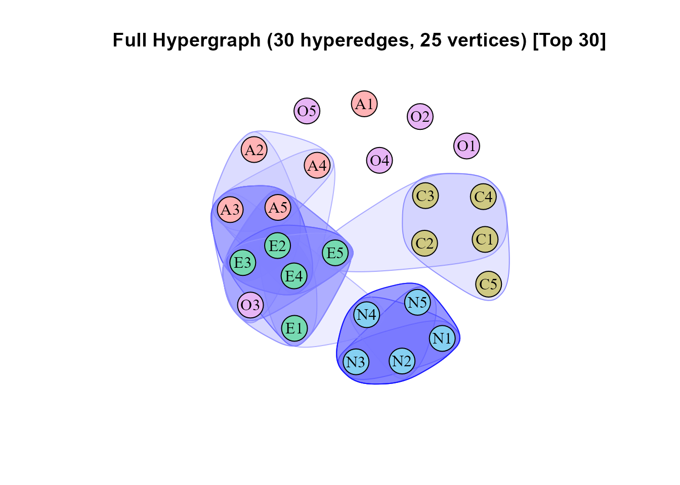

The 30 strongest retained hyperedges by absolute O-information. Node colors indicate theoretical item domains.

Shaded regions represent hyperedges. Red indicates negative O-information (synergy-dominated dependence), and blue indicates positive O-information (redundancy-dominated dependence). top_n changes the displayed selection, not the fitted object. Subsequent analyses of hg_bfi still use all 270 retained hyperedges. An uncluttered top-edge display need not include both signs.

plot(hg_bfi, type = "redundant", top_n = 20,
     groups = bfi_groups, vertex.size = 20, main = "Redundant hypergraph")
#> Selected top 20 hyperedges by absolute O-info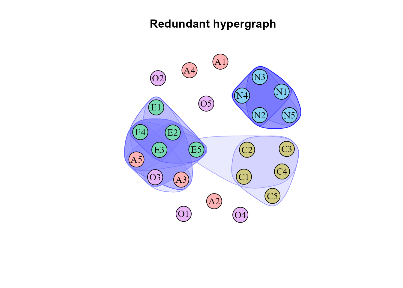

The 20 strongest redundant hyperedges in the reference fit.

plot(hg_bfi, type = "synergistic", top_n = 20,
     groups = bfi_groups, vertex.size = 20, main = "Synergistic hypergraph")
#> Selected top 6 hyperedges by absolute O-info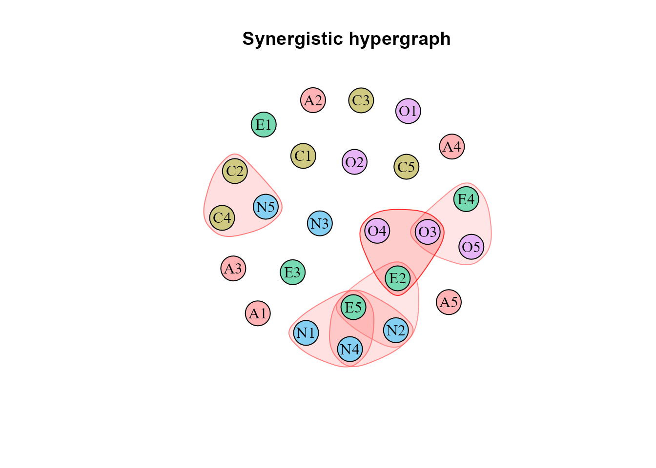

All six synergistic hyperedges retained in the reference fit.

The reference fit has only 6 synergistic hyperedges, so requesting its top 20 displays all 6. If a fitted object has no hyperedges of a requested type, the plotting method reports this instead of drawing that type. Color intensity is scaled separately within each displayed hypergraph; do not compare color darkness quantitatively across these panels.

plot_hyperedge(hg_bfi,
              significant_only = TRUE,
              show_edge_label = FALSE,
              point_size = 1)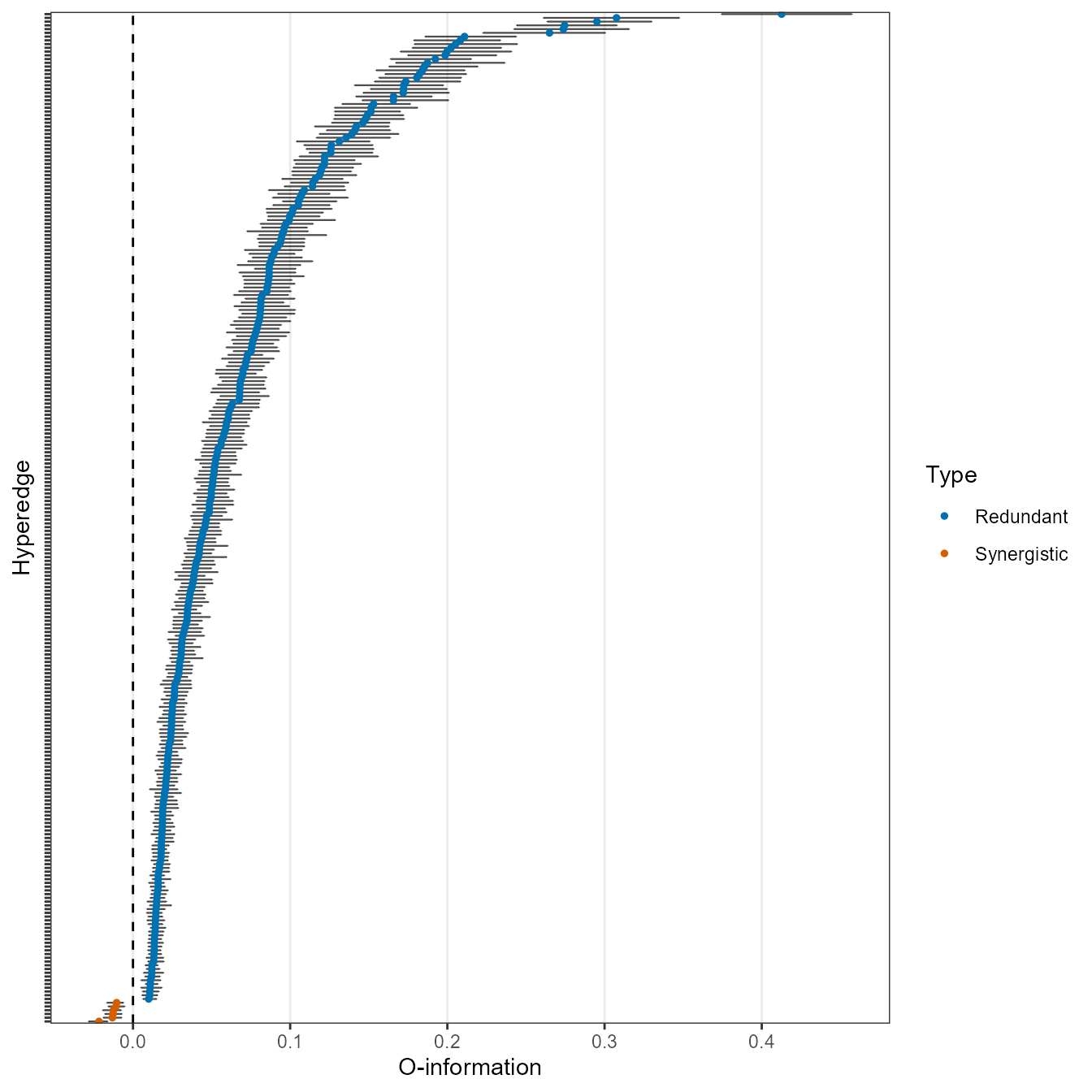

O-information estimates and BCa intervals for the 270 retained hyperedges. Most estimates are positive in this reference analysis.

The forest plot separates point estimates from their uncertainty. Points to the right of zero are redundancy-dominated. The predominance of positive estimates describes the retained structures under this estimator and search procedure.

5. Select a subset of existing hyperedges

Use subset_hypergraph() when you want to analyze or display a selected part of an existing fit without repeating the tests. Here we first restrict the orders and then keep the 20 strongest remaining hyperedges:

sub_hg <- subset_hypergraph(hg_bfi, k = 3:4)
sub_hg <- subset_hypergraph(sub_hg, top_n = 20)

sub_hg
#> psychHypergraph Object Summary
#> ==============================
#> 
#> Subjects: 2800
#> Variables: 25
#> Candidate Multiplets Evaluated: 20
#> Total Active Hyperedges: 20
#>   - Redundant (O-info > 0): 20
#>   - Synergistic (O-info < 0): 0
#> 
#> O-Info Statistics:
#>   Range: [0.139, 0.295]
#>   Mean (abs): 0.178
#> 
#> Parameters:
#>   cor_method: polychoric
#>   k: 3, 4, 5
#>   Candidate selection method: clique
#> 
#> Use $hypergraph to access full hyperedge list
#> Use $hyperedge_details to view complete test results
#> 
#> To plot:
#>   plot(x)                    # Full hypergraph
#>   plot(x, type='redundant')  # Only redundant
#>   plot(x, type='synergistic')# Only synergistic
#>   plot(x, top_n=10)          # Top 10 by |O-info|

The two calls make the order of operations explicit. In the current function, top_n is applied before k when both are supplied in the same call. The reference subset contains 20 redundant hyperedges, with O-information values approximately between 0.139 and 0.295 nats.

plot(sub_hg, groups = bfi_groups, vertex.size = 20)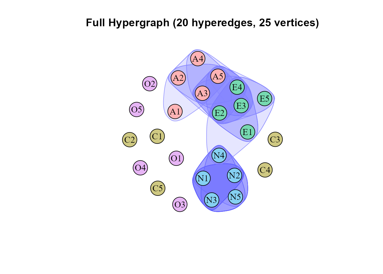

A subset containing the 20 strongest retained three- and four-item hyperedges.

The subset updates its hyperedge lists, incidence matrices, result table, and counts together. Its original_test_results field preserves the table from before the first subset operation. The printed settings still describe the original construction; a reduced row count after subsetting does not mean that only those rows were originally tested.

6. Examine node degree centrality

degree_bfi <- node_degree(hg_bfi)
head(degree_bfi)
#>   node_id node_name graph_type degree_type value
#> 1       1        A1  redundant      degree     5
#> 2       2        A2  redundant      degree    17
#> 3       3        A3  redundant      degree    32
#> 4       4        A4  redundant      degree    10
#> 5       5        A5  redundant      degree    49
#> 6       6        C1  redundant      degree    37

Degree is the number of active hyperedges containing a node. Weighted degree is the sum of the absolute O-information values of those hyperedges. Both are computed separately for redundant, synergistic, and full hypergraphs. For example, A5 participates in 49 redundant hyperedges in this reference fit.

plot_node_degree(hg_bfi,
                 graph_type = c("synergistic", "redundant"),
                 style = "both")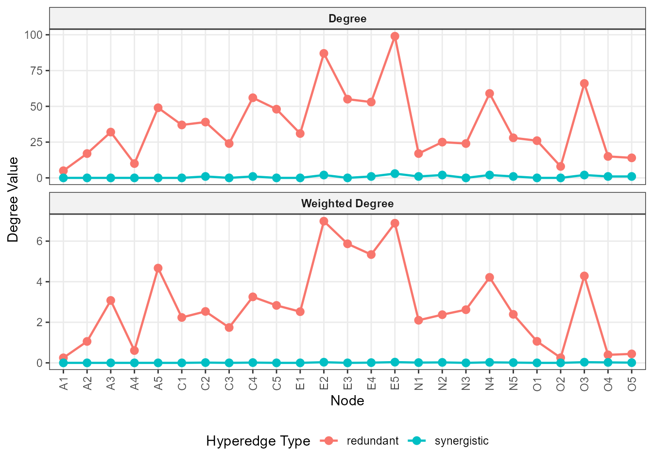

Raw degree and weighted degree in the redundant and synergistic hypergraphs.

plot_node_degree(hg_bfi,
                 scale = "relative",
                 graph_type = c("synergistic", "redundant"),
                 style = "both")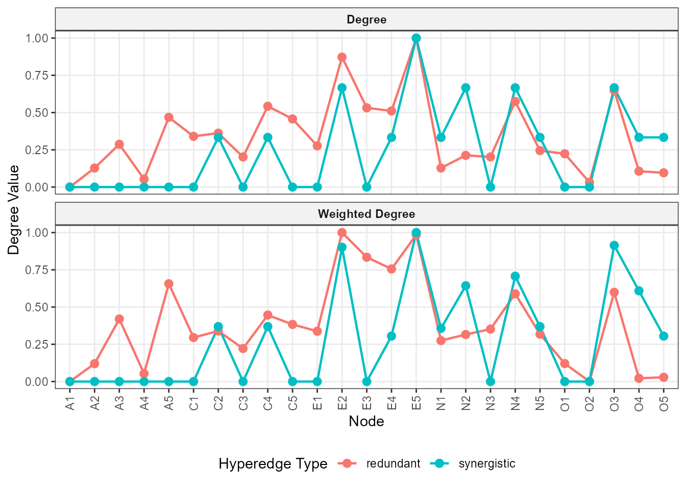

Degree measures after separate min-max scaling within each hypergraph type and degree measure.

scale = "relative" rescales each type of degree within each hypergraph type to the interval from zero to one. It is useful for comparing relative node profiles, but equal peaks do not imply equal absolute participation in redundant and synergistic structures. Use raw values to compare their magnitudes. Calling node_degree(sub_hg) instead would describe the selected subgraph, not the full fit. These measures quantify participation in the retained structures, rather than the effect of intervening on an item.

7. Cluster the nodes

Spectral clustering groups nodes according to their hyperedge participation. Here we choose five groups in advance to make comparison with the five item domains straightforward. The default weighted_l = FALSE uses a binary incidence representation.

clustering_result <- spectral_clustering(hg_bfi, K = 5, seed = 123)

clustering_result
#> Hypergraph Spectral Clustering Results
#> =====================================
#> Number of nodes: 25
#> Number of hyperedges: 270
#> Number of clusters (K): 5
#> Clustering method: Binary Laplacian
#> Non-isolated nodes: 25
#> Isolated nodes: 0
#> 
#> Cluster sizes:
#>   cluster size proportion
#> 1       1    4       0.16
#> 2       2    5       0.20
#> 3       3    6       0.24
#> 4       4    5       0.20
#> 5       5    5       0.20
#> 
#> First few eigenvalues:
#> [1] 0.0000 0.2404 0.3205 0.4348 0.5021
clustering_result$summary
#>   cluster size proportion
#> 1       1    4       0.16
#> 2       2    5       0.20
#> 3       3    6       0.24
#> 4       4    5       0.20
#> 5       5    5       0.20

cluster_table <- data.frame(
  item = names(data_bfi),
  domain = bfi_groups,
  cluster = clustering_result$membership
)

cluster_table
#>    item            domain cluster
#> 1    A1     Agreeableness       4
#> 2    A2     Agreeableness       4
#> 3    A3     Agreeableness       4
#> 4    A4     Agreeableness       4
#> 5    A5     Agreeableness       4
#> 6    C1 Conscientiousness       5
#> 7    C2 Conscientiousness       5
#> 8    C3 Conscientiousness       5
#> 9    C4 Conscientiousness       5
#> 10   C5 Conscientiousness       5
#> 11   E1      Extraversion       3
#> 12   E2      Extraversion       3
#> 13   E3      Extraversion       3
#> 14   E4      Extraversion       3
#> 15   E5      Extraversion       3
#> 16   N1       Neuroticism       2
#> 17   N2       Neuroticism       2
#> 18   N3       Neuroticism       2
#> 19   N4       Neuroticism       2
#> 20   N5       Neuroticism       2
#> 21   O1          Openness       1
#> 22   O2          Openness       1
#> 23   O3          Openness       3
#> 24   O4          Openness       1
#> 25   O5          Openness       1
table(cluster_table$domain, cluster_table$cluster)
#>                    
#>                     1 2 3 4 5
#>   Agreeableness     0 0 0 5 0
#>   Conscientiousness 0 0 0 0 5
#>   Extraversion      0 0 5 0 0
#>   Neuroticism       0 5 0 0 0
#>   Openness          4 0 1 0 0

The reference result broadly follows the item domains, but does not reproduce them perfectly: O3 is assigned to the group containing the extraversion items, while the other four openness items form a separate group. Cluster sizes are 4, 5, 6, 5, and 5. The labels themselves are arbitrary, and specifying K = 5 does not demonstrate that five is the best or automatically discovered number of groups.

split(cluster_table$item, cluster_table$cluster)
#> $`1`
#> [1] "O1" "O2" "O4" "O5"
#> 
#> $`2`
#> [1] "N1" "N2" "N3" "N4" "N5"
#> 
#> $`3`
#> [1] "E1" "E2" "E3" "E4" "E5" "O3"
#> 
#> $`4`
#> [1] "A1" "A2" "A3" "A4" "A5"
#> 
#> $`5`
#> [1] "C1" "C2" "C3" "C4" "C5"
head(clustering_result$membership_matrix)
#>      [,1] [,2] [,3] [,4] [,5]
#> [1,]    0    0    0    1    0
#> [2,]    0    0    0    1    0
#> [3,]    0    0    0    1    0
#> [4,]    0    0    0    1    0
#> [5,]    0    0    0    1    0
#> [6,]    0    0    0    0    1

The membership matrix indicates each node’s assigned group. A membership label of zero denotes an isolated node; the reference fit has none.

plot(clustering_result, type = "eigenvalues")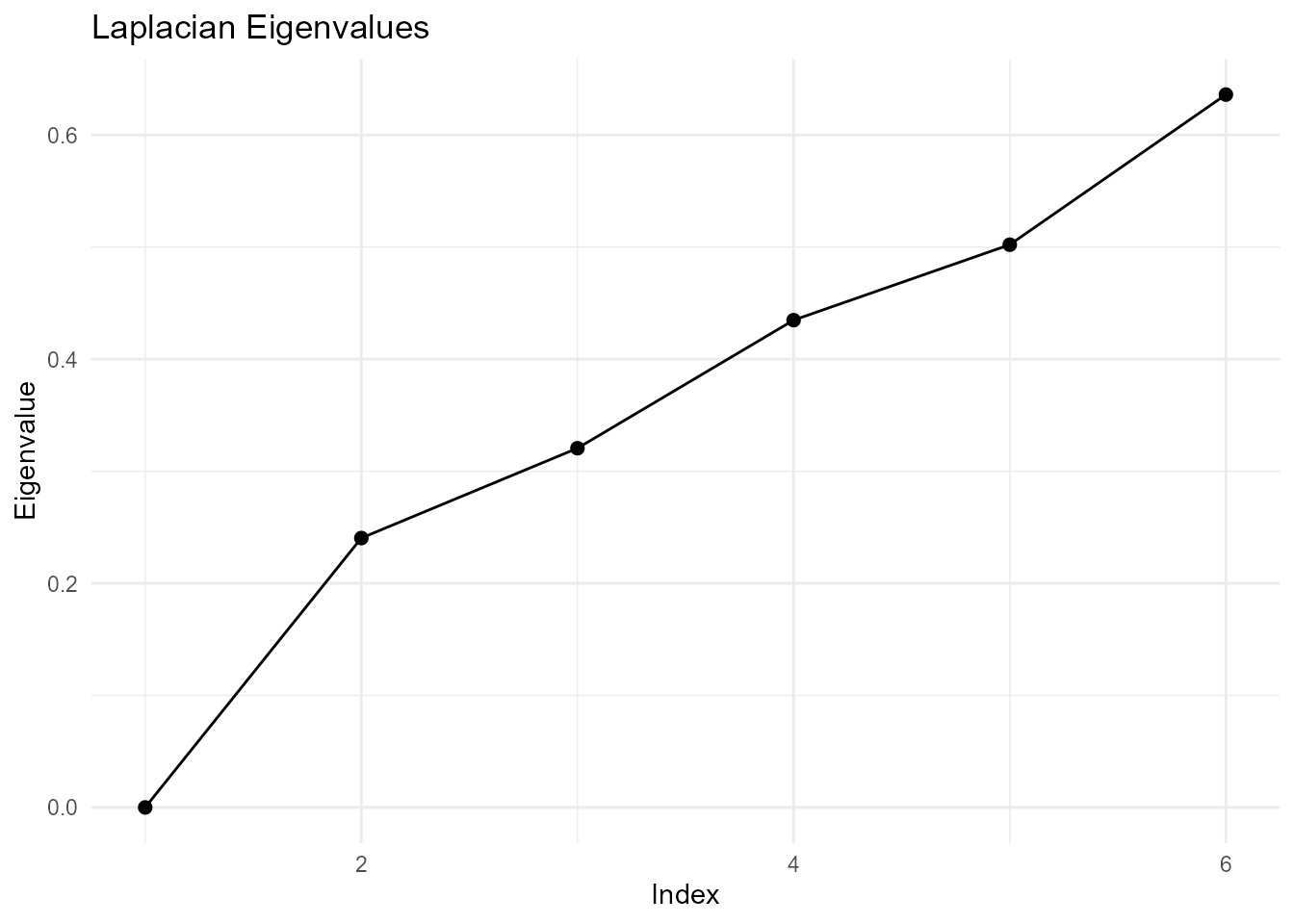

Laplacian eigenvalues associated with the spectral clustering example.

plot(clustering_result, type = "clusters")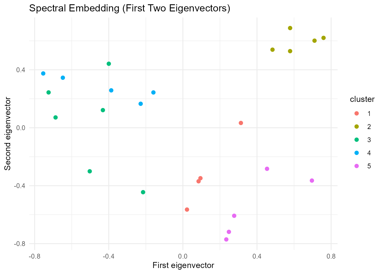

The first two coordinates of the spectral embedding, colored by the assigned groups.

The embedding plot is a two-dimensional view of the representation used for clustering.

plot(hg_bfi, top_n = 30, vertex.size = 20,
     groups = clustering_result$membership)
#> Selected top 30 hyperedges by absolute O-info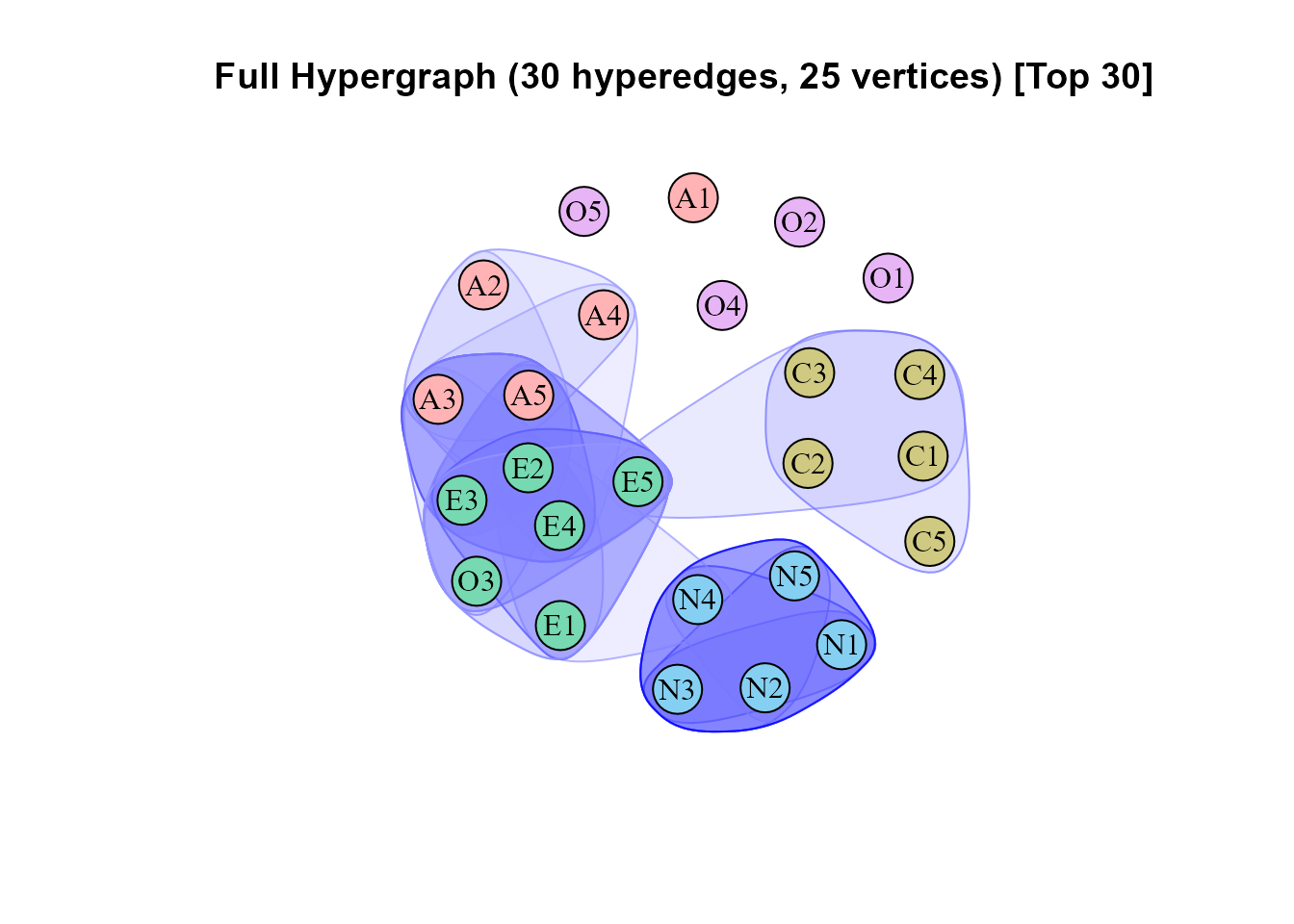

The 30 strongest retained hyperedges, with node colors now indicating spectral clusters.

8. Compare alternative correlation choices

Polychoric correlations can make the resampling workflow slow: they require estimating category thresholds and fitting latent correlations. Correlations are estimated repeatedly during permutation tests, bootstrap resampling, and BCa jackknife calculations. The package accelerates the jackknife step by reusing delete-one calculations for repeated response patterns, but repeated polychoric estimation can still be expensive. Pearson estimation is much faster in this application.

For computational efficiency, it can therefore be tempting to substitute Pearson for polychoric correlations. Before doing so, check whether the two workflows produce similar retained hyperedges and information estimates. This is a sensitivity check, not an assumption that the correlation models are interchangeable.

We now fit the Pearson alternative and compute the comparisons directly. The polychoric fit remains the saved reference object loaded above. Leaving transform = "auto" makes the alternative a rank-normalized Pearson workflow, not a Pearson analysis on the untransformed item values. As in the reference analysis, the low resampling counts below are for demonstration; increase them when assessing agreement for a research analysis.

hg_pearson <- build_hypergraph(
  data = data_bfi,
  cor_method = "pearson",
  k = 3:5,
  candidate_method = "clique",
  n_perm = 100,
  n_boot = 100,
  seed = 123,
  parallel = TRUE,
  n_cores = 12
)
#> Step 0/3: Preprocessing data...
#> Generating candidate multiplets using method: clique
#> Total candidate multiplets: 630
#> Step 1/3: Running permutation tests (n = 100)...
#> Step 2/3: Running BCa bootstrap validation (n = 100)...
#> Step 3/3: Running hierarchical validation...
#> Completed: Found 255 significant hyperedges.
#> Building hypergraphs...

hg_pearson
#> psychHypergraph Object Summary
#> ==============================
#> 
#> Subjects: 2800
#> Variables: 25
#> Candidate Multiplets Evaluated: 630
#> Total Active Hyperedges: 255
#>   - Redundant (O-info > 0): 254
#>   - Synergistic (O-info < 0): 1
#> 
#> O-Info Statistics:
#>   Range: [-0.013, 0.336]
#>   Mean (abs): 0.059
#> 
#> Parameters:
#>   cor_method: pearson
#>   k: 3, 4, 5
#>   Candidate selection method: clique
#> 
#> Use $hypergraph to access full hyperedge list
#> Use $hyperedge_details to view complete test results
#> 
#> To plot:
#>   plot(x)                    # Full hypergraph
#>   plot(x, type='redundant')  # Only redundant
#>   plot(x, type='synergistic')# Only synergistic
#>   plot(x, top_n=10)          # Top 10 by |O-info|

First compare the number of evaluated candidates and retained hyperedges:

data.frame(
  workflow = c("Polychoric", "Rank-normalized Pearson"),
  candidates = c(nrow(hg_bfi$all_test_results), nrow(hg_pearson$all_test_results)),
  retained = c(hg_bfi$n_hyperedges, hg_pearson$n_hyperedges),
  redundant = c(hg_bfi$n_redundant, hg_pearson$n_redundant),
  synergistic = c(hg_bfi$n_synergistic, hg_pearson$n_synergistic)
)
#>                  workflow candidates retained redundant synergistic
#> 1              Polychoric       1557      270       264           6
#> 2 Rank-normalized Pearson        630      255       254           1

Changing the correlation model can also change the estimated pairwise network used for clique search. Consequently, this comparison concerns the whole workflow, including candidate selection, not only the information estimator on a fixed set of multiplets.

After running both fits, match retained hyperedges by their variable combinations, rather than by their within-object IDs:

poly_edges <- hg_bfi$hyperedge_details[, c("vars", "k", "Oinfo")]
pearson_edges <- hg_pearson$hyperedge_details[, c("vars", "k", "Oinfo")]

jaccard <- function(a, b) {
  combined <- union(a, b)
  if (length(combined)) {
    length(intersect(a, b)) / length(combined)
  } else NA_real_
}

similarity <- do.call(rbind, lapply(c(NA_integer_, 3:5), function(order) {
  a <- poly_edges$vars[is.na(order) | poly_edges$k == order]
  b <- pearson_edges$vars[is.na(order) | pearson_edges$k == order]
  data.frame(
    order = if (is.na(order)) "Overall" else as.character(order),
    polychoric = length(a),
    pearson = length(b),
    shared = length(intersect(a, b)),
    Jaccard = jaccard(a, b)
  )
}))

print(similarity, row.names = FALSE)
#>    order polychoric pearson shared   Jaccard
#>  Overall        270     255    216 0.6990291
#>        3        156     132    126 0.7777778
#>        4         96      99     76 0.6386555
#>        5         18      24     14 0.5000000

The Jaccard index divides the number of shared edges by the number in their union. A value of one means identical edge sets, whereas zero means no shared edges. We return NA when both sets are empty. Comparing individual orders helps show whether agreement differs between triplets and larger groups.

Weights can also be compared on the shared edges:

common <- merge(
  poly_edges,
  pearson_edges,
  by = c("vars", "k"), suffixes = c("_poly", "_pearson")
)

rho <- if (nrow(common) >= 3 &&
           sd(common$Oinfo_poly) > 0 &&
           sd(common$Oinfo_pearson) > 0) {
  cor(common$Oinfo_poly, common$Oinfo_pearson, method = "spearman")
} else NA_real_

data.frame(
  shared_edges = nrow(common),
  Oinfo_Spearman = rho,
  sign_agreement = if (nrow(common)) {
    mean(sign(common$Oinfo_poly) == sign(common$Oinfo_pearson))
  } else NA_real_
)
#>   shared_edges Oinfo_Spearman sign_agreement
#> 1          216      0.9991891              1

Spearman correlation summarizes agreement in the ranking of shared-edge weights; sign agreement is the proportion assigned to the same redundancy/synergy type. Both are conditional on being retained by both workflows. They do not establish agreement on absent edges, equality of weight magnitudes, or equivalence of the two models.

Finally, visualize the overlap in the retained edge sets:

counts <- c(
  "Polychoric only" = length(setdiff(poly_edges$vars, pearson_edges$vars)),
  "Shared" = length(intersect(poly_edges$vars, pearson_edges$vars)),
  "Pearson only" = length(setdiff(pearson_edges$vars, poly_edges$vars))
)

bp <- barplot(counts, col = c("#4C78A8", "#59A14F", "#F28E2B"),
              ylab = "Number of hyperedges", main = "Hyperedge overlap",
              ylim = c(0, max(c(1, counts)) * 1.2))
text(bp, counts, labels = counts, pos = 3)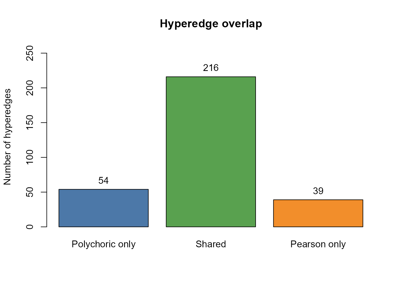

Retained hyperedges unique to each workflow and shared by both, calculated from the two fitted objects.

Use the overlap table, weight comparison, and substantive interpretation together to assess whether the faster workflow is adequate for the intended application. High shared-edge weight correlation can coexist with differences in which edges are retained. Neither computational speed nor a larger retained edge count alone establishes which model is appropriate.

9. Next steps and reporting

For a research application, report the analyzed variables and effective sample size; missing-value handling; correlation model and transformation; candidate strategy and orders; resampling counts, seed, and execution settings; adjustment method and thresholds; and any filtering or grouping used for presentation. Candidate coverage, effect size, order, sample size, and estimator assumptions all affect the results. More resampling improves Monte Carlo precision but does not replace additional participants. There is no universal sample-size threshold established by this example.

To specify candidate sets yourself, reuse fitted results by ID, or use an external node-clustering method, continue to Customize your own workflow.

sessionInfo()
#> R version 4.5.2 (2025-10-31 ucrt)
#> Platform: x86_64-w64-mingw32/x64
#> Running under: Windows 11 x64 (build 26200)
#> 
#> Matrix products: default
#>   LAPACK version 3.12.1
#> 
#> locale:
#> [1] LC_COLLATE=Chinese (Simplified)_China.utf8 
#> [2] LC_CTYPE=Chinese (Simplified)_China.utf8   
#> [3] LC_MONETARY=Chinese (Simplified)_China.utf8
#> [4] LC_NUMERIC=C                               
#> [5] LC_TIME=Chinese (Simplified)_China.utf8    
#> 
#> time zone: Asia/Shanghai
#> tzcode source: internal
#> 
#> attached base packages:
#> [1] stats     graphics  grDevices utils     datasets  methods   base     
#> 
#> other attached packages:
#> [1] psych_2.6.1           psychHypergraph_0.2.0
#> 
#> loaded via a namespace (and not attached):
#>  [1] tidyselect_1.2.1    dplyr_1.1.4         farver_2.1.2       
#>  [4] S7_0.2.0            fastmap_1.2.0       digest_0.6.37      
#>  [7] rpart_4.1.24        lifecycle_1.0.5     cluster_2.1.8.1    
#> [10] magrittr_2.0.4      compiler_4.5.2      rlang_1.2.0        
#> [13] Hmisc_5.2-5         sass_0.4.10         tools_4.5.2        
#> [16] igraph_2.2.1        yaml_2.3.10         data.table_1.17.8  
#> [19] knitr_1.51          labeling_0.4.3      htmlwidgets_1.6.4  
#> [22] mclust_6.1.2        mnormt_2.1.1        plyr_1.8.9         
#> [25] RColorBrewer_1.1-3  abind_1.4-8         foreign_0.8-90     
#> [28] withr_3.0.2         desc_1.4.3          nnet_7.3-20        
#> [31] grid_4.5.2          stats4_4.5.2        lavaan_0.6-21      
#> [34] future_1.67.0       colorspace_2.1-2    ggplot2_4.0.3      
#> [37] globals_0.18.0      scales_1.4.0        gtools_3.9.5       
#> [40] cli_3.6.5           rmarkdown_2.30      ragg_1.5.0         
#> [43] generics_0.1.4      otel_0.2.0          future.apply_1.20.0
#> [46] rstudioapi_0.18.0   RSpectra_0.16-2     reshape2_1.4.4     
#> [49] pbapply_1.7-4       cachem_1.1.0        proxy_0.4-27       
#> [52] stringr_1.6.0       parallel_4.5.2      base64enc_0.1-3    
#> [55] vctrs_0.6.5         boot_1.3-32         Matrix_1.7-4       
#> [58] jsonlite_2.0.0      glasso_1.11         Formula_1.2-5      
#> [61] htmlTable_2.4.3     listenv_0.10.0      systemfonts_1.3.1  
#> [64] jpeg_0.1-11         jquerylib_0.1.4     qgraph_1.9.8       
#> [67] parallelly_1.45.1   glue_1.8.0          pkgdown_2.2.0      
#> [70] codetools_0.2-20    stringi_1.8.7       gtable_0.3.6       
#> [73] quadprog_1.5-8      tibble_3.3.0        pillar_1.11.1      
#> [76] htmltools_0.5.8.1   R6_2.6.1            HyperG_1.0.0       
#> [79] textshaping_1.0.4   evaluate_1.0.5      pbivnorm_0.6.0     
#> [82] lattice_0.22-7      png_0.1-8           backports_1.5.0    
#> [85] corpcor_1.6.10      bslib_0.10.0        Rcpp_1.1.0         
#> [88] fdrtool_1.2.18      gridExtra_2.3       nlme_3.1-168       
#> [91] checkmate_2.3.3     xfun_0.56           fs_2.1.0           
#> [94] pkgconfig_2.0.3

This reports the environment used to render the vignette, not necessarily the original environment used to compute the saved reference fit.

References

Marinazzo, D., Van Roozendaal, J., Rosas, F. E., Stella, M., Comolatti, R., Colenbier, N., Stramaglia, S., & Rosseel, Y. (2024). An information-theoretic approach to build hypergraphs in psychometrics. Behavior Research Methods, 56, 8057-8079. https://doi.org/10.3758/s13428-024-02471-8

Possenti, F., Girelli, L., Tieri, P., & Petti, M. (2026). Multiplex Hypergraph Modeling of Higher Order Structures in Psychometric Networks. arXiv. https://doi.org/10.48550/arXiv.2604.22744

Rosas, F. E., Mediano, P. A. M., Gastpar, M., & Jensen, H. J. (2019). Quantifying high-order interdependencies via multivariate extensions of the mutual information. Physical Review E, 100, 032305. https://doi.org/10.1103/PhysRevE.100.032305